Criminal Classifier:
OpenCV based Criminal Identification Model
Introduction

In the realm of law enforcement and public safety, the Criminal Photo Classification and Visualization Project stands as a powerful tool, harnessing the capabilities of machine learning and computer vision technologies. I made this project to automatically identify and classify criminal individuals from images using a trained machine learning model. Leveraging OpenCV and the Haarcascade classifier algorithm, I explored various image processing techniques and conducted an analysis on the best model parameters, this system shows potential to empower law enforcement agencies with an efficient means of sorting and visualizing data related to known criminals.
Methodology
Data Loading and Exploration: A diverse dataset containing images of individuals labeled with their respective criminal identities, such as Al Capone, Dawood Ibrahim, Osama Bin Laden, and Pablo Escobar was loaded visualize to gain an understanding of the dataset’s structure, quality, and content.
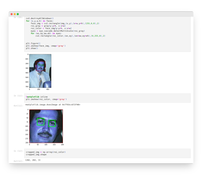
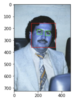
Face and Eye Detection: Implemented Haarcascade classifiers for face and eye detection to identify and extract facial features, an essential step in criminal identification. (Fig. 1)
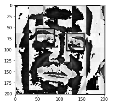
Data Pre-Processing: Cropped images based on detected faces and eyes were saved, ensuring that each image contains the necessary features for classification. Wavelet transformation was applied to the cropped images, extracting features from both raw and transformed images to enhance the model’s ability to capture intricate patterns followed by data augmentation. (Fig. 2)


import numpy as np
import cv2
import matplotlib
from matplotlib import pyplot as plt
from sklearn.svm import SVC
from sklearn.preprocessing import StandardScaler
from sklearn.model_selection import train_test_split
from sklearn.pipeline import Pipeline
from sklearn.metrics import classification_report
%matplotlib inline

img = cv2.imread('./Documents/CriminalClassifier/model/dataset/Pablo Escobar/8.jpg')
plt.imshow(img)

img.shape
gray = cv2.cvtColor(img, cv2.COLOR_BGR2GRAY)
gray.shape

# Loading Haarcascades
face_cascade = cv2.CascadeClassifier('./haarcascade_frontalface_default.xml')
eye_cascade = cv2.CascadeClassifier('./haarcascade_eye.xml')

faces = face_cascade.detectMultiScale(gray, 1.3, 5)
faces

(x,y,w,h) = faces[0]
x,y,w,h
face_img = cv2.rectangle(img,(x,y),(x+w,y+h),(255,0,0),2)
plt.imshow(face_img)

# Visualizing Face and Eye detection
cv2.destroyAllWindows()
for (x,y,w,h) in faces:
    face_img = cv2.rectangle(img,(x,y),(x+w,y+h),(255,0,0),2)
    roi_gray = gray[y:y+h, x:x+w]
    roi_color = face_img[y:y+h, x:x+w]
    eyes = eye_cascade.detectMultiScale(roi_gray)
    for (ex,ey,ew,eh) in eyes:
        cv2.rectangle(roi_color,(ex,ey),(ex+ew,ey+eh),(0,255,0),2)


plt.figure()
plt.imshow(face_img, cmap='gray')
plt.show()

# Cropping ROI
def get_cropped_image_if_2_eyes(image_path):
    img = cv2.imread(image_path)
    gray = cv2.cvtColor(img, cv2.COLOR_BGR2GRAY)
    faces = face_cascade.detectMultiScale(gray, 1.3, 5)
    for (x,y,w,h) in faces:
        roi_gray = gray[y:y+h, x:x+w]
        roi_color = img[y:y+h, x:x+w]
        eyes = eye_cascade.detectMultiScale(roi_gray)
        if len(eyes) >= 2:
            return roi_color

# Wavelet Transform
def w2d(img, mode='haar', level=1):
    imArray = img
    #Datatype conversions
    #convert to grayscale
    imArray = cv2.cvtColor( imArray,cv2.COLOR_RGB2GRAY )
    #convert to float
    imArray =  np.float32(imArray)
    imArray /= 255;
    # compute coefficients
    coeffs=pywt.wavedec2(imArray, mode, level=level)

    #Process Coefficients
    coeffs_H=list(coeffs)
    coeffs_H[0] *= 0;

    # reconstruction
    imArray_H=pywt.waverec2(coeffs_H, mode);
    imArray_H *= 255;
    imArray_H =  np.uint8(imArray_H)

    return imArray_H

# Model I/p O/p
X, y = [], []
for criminal_name, training_files in criminal_file_names_dict.items():
    for training_image in training_files:
        img = cv2.imread(training_image)
        scalled_raw_img = cv2.resize(img, (32, 32))
        img_har = w2d(img,'db1',5)
        scalled_img_har = cv2.resize(img_har, (32, 32))
        combined_img = np.vstack((scalled_raw_img.reshape(32*32*3,1),scalled_img_har.reshape(32*32,1)))
        X.append(combined_img)
        y.append(class_dict[criminal_name])

# Model Training
X_train, X_test, y_train, y_test = train_test_split(X, y, random_state=0)

model_params = {
    'svm': {
        'model': svm.SVC(gamma='auto',probability=True),
        'params' : {
            'svc__C': [1,10,100,1000],
            'svc__kernel': ['rbf','linear']
        }
    },
    'random_forest': {
        'model': RandomForestClassifier(),
        'params' : {
            'randomforestclassifier__n_estimators': [1,5,10]
        }
    },
    'logistic_regression' : {
        'model': LogisticRegression(solver='liblinear',multi_class='auto'),
        'params': {
            'logisticregression__C': [1,5,10]
        }
    }
}


scores = []
best_estimators = {}
import pandas as pd
for algo, mp in model_params.items():
    pipe = make_pipeline(StandardScaler(), mp['model'])
    clf =  GridSearchCV(pipe, mp['params'], cv=5, return_train_score=False)
    clf.fit(X_train, y_train)
    scores.append({
        'model': algo,
        'best_score': clf.best_score_,
        'best_params': clf.best_params_
    })
    best_estimators[algo] = clf.best_estimator_

df = pd.DataFrame(scores,columns=['model','best_score','best_params'])
dfModel Training & Evaluation: The features were inputted to different machine learning models, including Support Vector Machines (SVM), Random Forest, and Logistic Regression. GridSearchCV was used to identify the best model and fine-tune the hyperparameters (Code Block above). Lastly the model was exported and tested on a small dataset of test images.
Results & Discussion
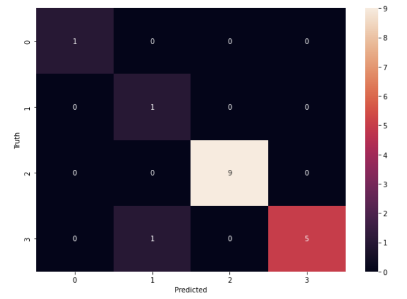
The results showed that the Support Vector Machine with the parameters: {‘svc__C’: 1, ‘svc__kernel’: ‘linear’}, performed the best with an accuracy of 90% as compared to random forest and logistic regression models. The confusion matrix below shows the classification results for each class (each criminal) on a very limited dataset. The exported model was later tested in a real-time setting where the printed images of the criminals were placed in front of the web-cam to detect and predict the image frames in real-time.


Conclusion & Future Work
The Criminal Photo Classification and Visualization Project successfully demonstrated the efficacy of machine learning and computer vision in identifying and classifying criminal individuals. The model, trained on a diverse dataset, exhibited strong performance, paving the way for potential applications in law enforcement. Future endeavors could involve expanding the dataset to encompass a wider range of criminals, enhancing model interpretability, and integrating real-time image processing for dynamic criminal identification scenarios. Additionally, exploring advanced deep learning architectures and collaborating with law enforcement agencies can contribute to further refinement and deployment of this technology.
Additional Documents
More detains about this project: Github Link.
Guide: –